The Experiment in Applying 3D
Technology of Magnetic Fields Interpretation at the archaeological site
“Arkaim”
V. Kochnev*, G.Zdanovich**, B. Punegov**
*Institute of Computational Modeling SB RAN,
Krasnoyarsk.
**Historical Center “Arkaim”, Chelyabinsk.
chelyabinsk@aces-group.com, kochnev@icm.krasn.ru
Prerequisites of the experiment
Arkaim, the fortified settlement dated to 1600–1700 B.C., was discovered in 1987 [1]. It is situated 8.2 km north–north–west of Amurskiy, and 2.3 km south–south–east of Alexandronvskiy in the Chelyabinsk region, Russia. “The excavation revealed that the settlement had been burned and, therefore, many details were preserved. The population, however, had vacated the city before the fire and took all their possession with them. Arkaim had two protective circular walls and two circles of standard dwellings separated by a street around a central square. The external wall, 160 m in diameter and 4 m wide, was built from specially selected soil that had been packed into timber frames before being faced with adobe bricks. On the interior, houses abutted the wall and were situated radially with their doors exiting to the circular internal street.” [7] The site plan is shown at Fig.1.
It is
known from experience that the interpretation of magnetic fields and some of
their components gives good results in the detection of archaeological objects
without actual excavations. The differences in the magnetic susceptibility of
the building material of walls, soil and gumus that covered the archaeological
object are crucial for the successful detection. That fact was proved by the
application of magnetic fields on the archaeological site «Arkaim» . We made an
attempt to start the construction of the model of the magnetic properties of
medium under the surface. For this purpose we used the technology, developed by
us for studying different geological objects [4,6].
The software package ADGM-3D is the core element of the technology that makes it possible to calculate magnetic and gravitational fields from known objects generating fields (direct problem), and the parameters of objects from the observed anomalous fields (inverse problem).
The model of medium and the
method of the solution
For the solution of these problems we assumed a block-layered model with rectangular parallelepipeds as elementary objects. The lateral dimensions of parallelepipeds for the entire site are the same and are determined by the observation grid. The vertical dimensions are predetermined by the boundaries of layers. We used well-known formulas [2] for the solution of the direct problem. For the inverse problem the adaptive method of solving the systems of algebraic (linear and nonlinear) equations [3,4,5] was applied. The method does not accumulate errors and makes it possible to solve the systems with a large number of equations and unknowns quantities.
Initial data
Let’s move on to the object under study. In Fig.1 we can see the model of «Arkaim» site and the fragment which we used for the experimental interpretation (red lines). The Northwestern segment was excavated earlier, but the eastern part was not, including the area of our research. Fig.2 shows the area relief of the studied fragment. The survey of magnetic field was conducted on the grid of 0.5x0.5 m. The dimensions of the studied fragment are 30x40 m. The number of points is 61x81=4941.
The initial magnetic field (in 10-colors palette) is shown in Fig.3. Negative values are in red colors, positive – in dark-blue. We can see two strips of positive anomalies which coincide with the direction of convex relief forms. The limits of the field vary from –116 to 123 nT. Rectangular forms of slight positive anomalies can be discerned in the background (in dark green) We can also single out two strong anomalies of the complex form. The first is located in the central part (profile 0), the second one is situated to the north. (It should be taken into consideration that the anomalies go from South to North almost bias from the bottom left corner to the top right corner) On the profile –1500 we can see a negative anomaly, caused by a natural deepening. Two areas with the calm field (yellow spots in the lower and central parts of the figure) should also be focused at.
Solution of the inverse problem
In order to solve the inverse problem it is necessary to assign the initial approximation of model. The solution can be found while applying the problem to the single-layer model, but it proves to be unstable. Minimum discrepancy occurs at the first iteration, but it increases at the iterations following the first one. (Discrepancy is the difference between the original and modeled values of field). After a number of experiments, we accepted the three-layered model of medium with the boundaries of the layers imitating the surface relief. The layers were 30, 60 and 120 cm thick. Thus, the total thickness of model was 210 cm. It was assumed that magnetic susceptibility for all layers is 50*10-5 SI, and the initial approximation error is 10*10-5 SI.
The following discrepancies were obtained in the process of solving the inverse problem:
9.7 5.2 3.9 3.1 2.6 nT.
In 1 hour we obtained the 3-layer model of magnetic susceptibility for the entire area of study. Fig. 4 shows the magnetic field, calculated from the model. It is almost undistinguished from the initial field. The proximity of the initial and the model magnetic fields suggests that one of the possible solutions is obtained.
Analysis of the results
In Fig.5 we see the magnetic susceptibility of the first layer. It changes from 4 to. 92*10-5 SI. At the picture we can distinctly see those special features of the forms which were visible in the magnetic field. Emphasized parts are regions of calm (not technogenic) fields in light green, yellow and red colors.
The distribution of the magnetic susceptibility in the second layer is shown in Fig.6. One can trace here the same features noted before but in a smoother form. The magnetic susceptibility of the third layer (shown here in the individual local palette) we can see in Fig.7. The range is from 28*10-5 to 51*10-5 SI.
Let us further look at the most interesting sections first in the left-to-right, and then in the bottom-to-top direction. On the upper sequence of Fig.9 we see a section along the profile –1500, passing through a negative anomaly, which is located to the south of the bank. Note two specific features. The upper layer has high magnetic susceptibility while the lower level is characterized by low magnetic susceptibility. This is especially visible in the area of the decline in the relief.
The second sequence presents a section along one of the positive anomalies. Two parts with the increased magnetic susceptibility are noted here: in the center and on the right. Moreover the first one corresponds to the negative form of relief, and the second one - to the positive. The third sequence shows a section along profile +500. In the cavity on the left a reduction in the value of magnetic susceptibility can be seen. Note that the lowered regions of relief both beyond the boundary of the fortress (sequence 1) and within the limits of the fortress (sequence 3) have lowered values of magnetic susceptibility with smooth changes. Does that indicate that in this part of the fortress there are no walls of dwellings or some other constructions? Could it be a small reservoir inside the fortress, surrounded by trees?
Fig. 9 shows profiles that pass from the lower part of the section to the upper. All special features, indicated on the left-to-right profiles, are visible here as well. Fig. 8 shows the three-dimensional model of the object with somewhat different variants of visualization.
The experimental processing of 4-level observations
In the small section of 20x1.5 m geophysicists carried out the survey of magnetic field on 4 levels: on the surface, 5, 15 and 25 cm above the surface with a sampling interval 50 cm. The initial and modeled magnetic fields are shown in Fig.11, initial and modeled curves are in Fig.12. Let’s look at sections (Fig.13) and compare them with the results obtained with level 1of the survey (Fig.14). They somewhat differ.
Let’s do the calculation of the magnetic field at 7 levels, imitating the surface. The first is on the surface, and the last is at height of 3.5 m. We can see that the magnetic field at latter two levels is close to 0. Analyzing the results of simulation we come to the conclusion that the optimum level of observation could be 0, 15, 30 or 60 cm.
Brief description of the technology
The software package ADGM-3D serves as the basis of the technology. The number of profiles, points, layers and the number of observation levels are unlimited. The rapid and stable method of solving inverse problems in combination with the graphic possibilities gives the possibility to solve complex problems. All illustrations in this paper were obtained with the graphic means of the package.
Conclusion
We obtained a 3-layer, 3-dimensional model of magnetic susceptibility of a near-surface part up to 210 cm in depth (30x40 m) of the archaeological site “Arkaim”. This approach enabled us to compose maps of each layer and sections along different paths. We show 6 sections, crossing characteristic anomalous zones. Zones with strong and weak fluctuations of susceptibility were identified on maps and sections. 3 strong anomalies were found. First – negative, beyond the fortress limits, correlated with local lowered form of relief and probably connected with the burial site. Two other ones are positive, inside the fortress, probably connected with ancient metallurgy items.
Data from 4-level survey of 20x1.5 m part were processed. These data turned out to be higher. We would recommend to use this technology advantages for choosing an optimal survey scheme
The first experiment of the application of this technology showed that there are many interesting tasks in the field of archaeology to be worked at by geophysics and archaeologists in cooperation. We should not forget that magnetometry is a rather precise and highly productive method and at the same time comparatively simple in application. Topographic survey and mapping are the most laborious part of such works. One of the tasks for archaeologists is to analyze the results of experimental interpretation with the aid of our technology, which was created for solving forward and inverse problems in geology. We worked on this problem with great interest and enthusiasm.
Special thanks
The authors thank the co-authors of the package D.Vasil'ev and V.Sidorov for the collaboration, and also I.Goz., M.Starikova for the help in preparing and translating the work.
References
1.Arkaim (studies and explorations). Chelyabinsk, 1995.
2.Aleksidze M.A. Approximation methods for solving forward and inverse gravimetric problem. - Moscow, Nauka, 1987. - 336 p.
3.Kochnev V.A. Adaptive methods of interpreting seismic data. - Novosibirsk, Nauka, 1988. - 152 p.
4.Kochnev V.A. Adaptive methods of solving inverse geophysical problems. - Krasnoyarsk, Comp.Center of SB RAN, 1993.
5.Kochnev V.A., Khvostenko V.I. Adaptive methods of solving inverse gravimetric problem. Geologiya i geofizika, 7, 1996. p.120-129
6.Kochnev V.A., Vasiliev D.V., Sidorov V.Y. The technique of solving 3-D gravity problems. SEG International Exhibition, Salt Lake City, 2003.
7.Koryakova L. Sintashta-Arkaim Culture, http://www.csen.org/koryakova2/Korya.Sin.Ark.html
figure 1 – Archaeological site “Arkaim” (research area
is shown in rectangle)
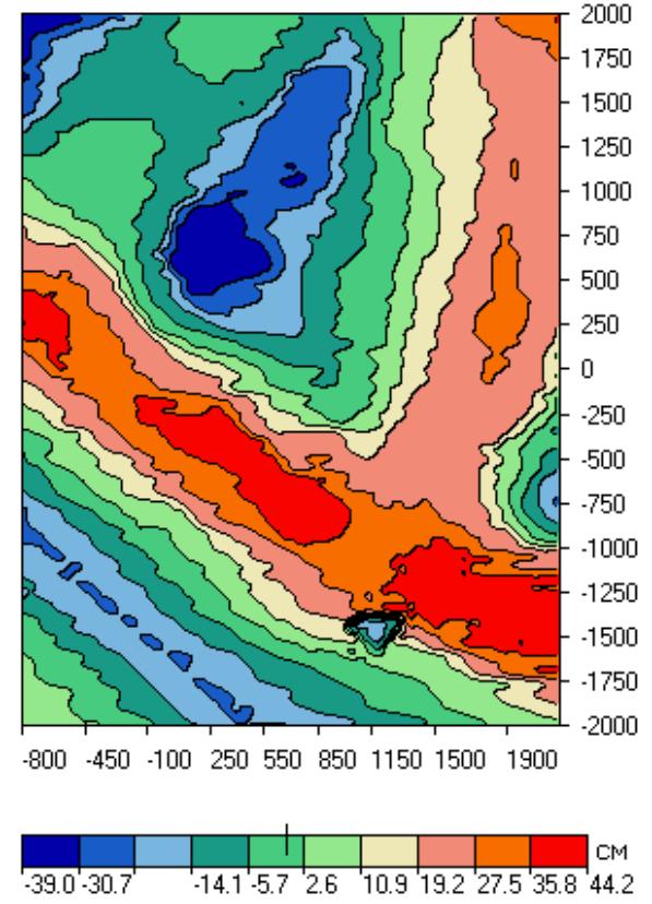
figure 2 – The relief of research area
figure 3 – Initial anomalous magnetic field observed at
the surface
figure 4 – Modeled magnetic field
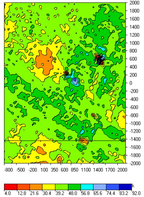
figure 5 –
Magnetic susceptibilities for the first layer
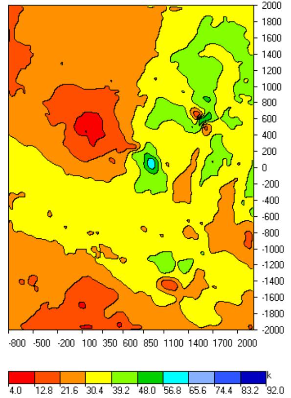
figure 6 – Magnetic susceptibilities for the second
layer

figure 7 – Magnetic susceptibilities for the third
layer
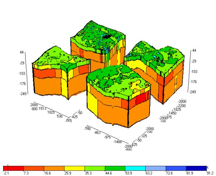
figure 8 –3D model (block variant)
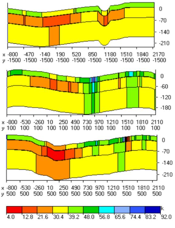
figure 9 – SW-NE sections along profiles –1500, 100 и 500
figure 10 – NW-SE sections along lines on 950, 1150,
1550 pickets.
figure 11– Magnetic fields. Initial (left), modeled
(right)
figure 12 – First row: plots, second row: fields.(left:
initial, roght: modeled), third row: sections, visualized in isolines and
block-style
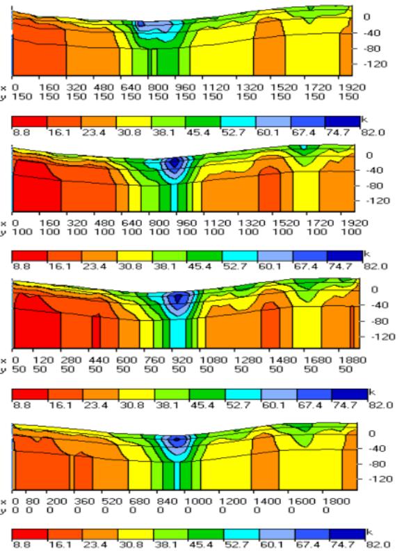
figure 13 – Magnetic susceptibilities sections 4,3,2,1
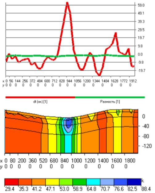
figure 14 – Plot of magnetic field along latitudial
profile 100 (dt[ок]–initial and differencial) and section obtained from
one-level data.
figure 15 – Magnetic fields, profile 100. From up to
down: plots and section of observed field, plots and section modeled on 7
levels.