Packet is intended for the solution of the forward and inverse three-dimensional and two-dimensional problems of magnetometry based on the data of the anomalous magnetic field, measured in the knots of uniform grid on the assigned surfaces of observation.

Algorithm

Three-dimensional block-layered model of medium with the piecewise-linear layer boundaries is assumed for the purposes of solution. Each layer is approximated by the set of parallelepiped elements (blocks). Along the axes X and Y the partition into the blocks is conducted according to the preset rectangular grid, while the vertical dimensions of blocks are determined by the positions of layer boundaries. Inside of the elementary block the magnetic susceptibility of medium assumed constant.

We consider the following problems:

a) For each elementary block, value of the magnetic susceptibility is given. All boundaries are known. Determine the values of DT_a or DZ_a along the required surfaces, which can coincide or not with the original ground.

b) The values of DT_a or DZ_a are given. All boundaries are known. Determine the magnetic susceptibilities for each block.

c) The values of DT_a or DZ_a are given and for each elementary block, value of the magnetic susceptibility is given. Also, the upper and bottom boundaries are known. Determine the inner layer boundary positions.

It is customary in geophysics to call the problems subsequently forward problem, inverse problem and contact problem. Adding up magnetic influences from each elementary block solves the forward problem. The field of elementary block calculated from known formulae [1,2]. The inverse problem is reduced to solving a linear equation system, and the contact problem is described by non-linear equation system, where coefficients are dependent of the layer boundary coordinates. Both systems are solved by adaptive method of solving the systems of algebraic (linear and nonlinear) equations. The coefficients of system in contact problem are refined after each iteration.

The adaptive method being used has the following features:

it uses the initial approximations of unknown susceptibilities (or boundaries);
takes into account their a prioi possible errors (APE). Changing APE influences resultant parameter values. Enlarging APE results in broader range for parameter value searching and vise versa. Zeroing APE will fix parameter value in place;
doesn’t accumulate errors, which allows for a solution of the systems with a large quantity of equations and unknowns;
allows finding solution that is the closest to a priori set one in the case when the problem has multiple solutions.

The solution of inverse problem gives a block model with completely determined susceptibilities, boundaries and modeled field. After that, we can solve additional problem of finding layer-homogeneous model with double number of layers. Each layer will be divided onto two sub-layers, assuming that susceptibilities are constant within those sub-layers. The upper sub-layer will be assigned minimal value from all the blocks making up the layer and the bottom sub-layer will receive maximal. Then, a new boundary position will be calculated so that summated magnetic moment from both blocks equaled that from old block. It is also possible to manually choose susceptibilities of sub-layers and boundary position. That new model can later be used as an initial approximation for the contact problem. Finally, anomalous gravity field Dg will be calculated.

Input data

The input data contain information about model geometry, physical properties of medium, computation variants and conditions and also some text information about researched field and well logs. Each piece of data has a designation., which are used in table descriptions and help system.

Two main types of input data are scalars and arrays.

Scalars

This type of parameter represents a simple scalar value.

Tasks. This parameter can assume four values:

None, which means that no task is selected
Forward – forward problem will be solved
Inverse – first, inverse problem will be solved, then, according to obtained susceptibilities values, model magnetic field will be computed
Contact – you guessed it, contact problem will be solved, then, according to obtained boundary positions, model magnetic field will be computed

As you can see, forward problem will always be solved after inverse problem. If you set Iterations at 0, inverse problem solution will be skipped. It is a convenience feature, intended for use with manual inverse problem solution. According to this method, you do not compute model parameters, but change them manually. Of course, this method can reasonably be used only for very simple task.

Number of…

Layers – number of layers in model. Unlimited. It is recommended, though, do not exceed 20 layers per model.
Profiles – number of elementary blocks along X axis (unlimited)
Points in profile – number of elementary blocks along Y axis (unlimited)
Iterations – number of iterations for solution of inverse or contact problem
Curves – number of survey levels. Unlimited, but more than 10 is probably not very effective

Model parameters

Distance between points – survey data grid step along Y-axis, meters
Distance between profiles – survey data grid step along X-axis, meters

Above parameters are determining the dimensions of elementary blocks.

Inner radius, outer radius (meters). Solving problems with high number of layers and blocks can be time-consuming. We can accelerate the solution, if for each observation point will ignore all blocks situated further than “inner radius”. “Outer radius” controls the area for blocks participating in divider computation. Outer radius must be greater then inner radius. If both radiuses are greater then maximal diagonal size of the research area, computations will be precise. Forward problem always computed exactly. It is better to keep inner radius close to actual distance between observation points.
X normal component – the strength of background magnetic field along X-axis, Oe.
Y normal component – the strength of background magnetic field along Y-axis, Oe.
Z normal component – the strength of background magnetic field along Z-axis, Oe. These parameters characterize the normal Earth magnetic field strength at the research area. Induced magnetization of each elementary block computed as: J_xijk =k_ijk·X; J_yijk =k_ijk·Y; J_zijk =k_ijk·Z, where k_ijk – magnetic susceptibility of block in layer i, profile j, point k.
Noise – additive noise level for forward problem
Iterations – number of iterations for inverse or contact problem. Should be 1. If >1, then kapx[k] will replace kap0[k], thus erasing initial data. Then, s0[ок] and skap[о] will be halved and computation will be run again.

Data description

Object description – any sequence of symbols no longer then 60 symbols.

Scale – any sequence of symbols no longer then 60 symbols.

You can use these fields to designate field name and scale of data.

Input arrays

Each of the following arrays shown as a matrix of kp*kt dimensions. Value in square brackets shows a type of task, for which this array applied.

п – forward

о – inverse

к – contact

z[по] – Boundaries. Levels in meters. Levels below sea level are negative numbers. First boundary - sensor level, last - bottom of downmost layer.

kapx0[о] – Initial estimation of susceptibilities. For inverse problem.

skap0[о] – Error estimations of susceptibilities values. For inverse problem.

zx0[к] – Initial estimation of boundary coordinates. For contact problem.

sz[к] – Error estimations for boundary coordinates. For contact problem.

kap[пк] – Susceptibilities (kappa). Absolute or excessive values for each layer. Used in forward and contact problem.

dt[ок] – Observed magnetic field anomalies, nT. For inverse and contact problems.

dx_rk[ок] – Strengths of observed magnetic field anomalies along X-axis, nT For inverse and contact problems.

dy_rk[ок] – Strengths of observed magnetic field anomalies along Y-axis, nT For inverse and contact problems.

dz_rk[ок] – Strengths of observed magnetic field anomalies along Z-axis, nT For inverse and contact problems.

s0[ок] – Mean square error of magnetic field anomalies.

un[пок] – For each observation curve, level (meters) for recalculating magnetic field anomalies from model estimated as a result of inversion or contact problem. Levels below sea level are negative numbers.

Fij – Background susceptibilities. Must be set for each layer, if it is desirable to obtain absolute (not excessive) susceptibilities. Otherwise, must be 0.

Typk – Curve type of anomalious field. 0–curve not used, 1–DHx,2–DHy, 3–DHz, 4–Dt.

For joint interpretation of magnetic and gravity data the following parameters must also be set:

Bk – ks constants (meters per sec. per susceptibility unit).

Vk – ks constants (meters per sec. per susceptibility unit).

Density for k-layer and i,j-block is calculated as: ro[k,i,j] = bk[k]*ln(kap[k,i,j]) + vk[k].

Calculated densities are used for forward gravity modeling. Computation can be performed either alongside with forward problem solution, or by selecting Compute->Misc.

fij_gr – Background densities. Must be set for each layer, if it is desirable to obtain absolute (not excessive) densities.

Output arrays

You probably wonder what array with strange name “---------“ in the list means. This is buffer array, separating input data from output and can also be used for exchanging data between arrays at will.

nevz[пок] – Mean square discrepancies between observed dt and calculated from model obtained as a result of inversion or contact problem.

kapx[о] – Susceptibilities, results of inversion.

skapx – Susceptibility error estimates obtained from inversion.

zx[к] – Boundaries, results of contact problem solving.

szx[k] – Boundary coordinates error estimates. Obtained from contact problem.

dt[п]– dt field values from forward problem. Also, from a model obtained as a result of inversion or contact problem.

Разность – Magnetic field error estimates (any problem)

dx_l[п] – dT field values along X-axis, obtained from the solution of forward problem. Also, from the forward modeling of data from inverse or contact problem.

dz_l[п] – dT field values along Z-axis, obtained from the solution of forward problem. Also, from the forward modeling of data from inverse or contact problem.

dy_l[п] – dT field values along Y-axis, obtained from the solution of forward problem. Also, from the forward modeling of data from inverse or contact problem.

ro – Densities for each layer. Excessive or absolute values. For forward gravity problem.

dg[п] – dg field values, obtained from forward modeling of gravity from results of inversion, converted to densities.

Operating manual

The main operating modes of ADGM-3D are: creating, reading, editing and checking job files, running computation and visualizing results.

Main menu

Main menu is always available in upper part of program window. There are 6 sub-menus: File, Orientation, Compute, Settings and Help.

File – groups together commands for working with job files:

New – creates new job with no input data
Import – creates new job and fills it with data from imported grid file. The dimensions of the model will be determined by grid file.
Open – opens saved earlier job file from the disk. All current non-saved data will be thrown away.
Save – saves current job into a file, overwriting its contents.
Save as – prompts for a file name and saves current job
Export – exports arrays to a grid file. The file will contain coordinates of points and data values. You will be prompted for filename.
Batch mode – you can stack up several jobs and run them sequentially.
Exit – you guessed it, exit from program.

Orientation – transpose model data. Select from 90 deg. clockwise, mirror vertical (interchange east and west) and Auto (program will try to guess correct orientation based on X,Y data). Coordinates of points will not be changed.
Compute – run the computation

New computation – run from the beginning
Continue computation – continue computation if it was interrupted
Misc – compute densities and anomalous gravity field

Windows – show/hide different windows. One of them contains event log, others are refer to graphics.

Images: Basic settings – change plot name, level number, number of isolines, display of isolines and logs.
Images: Size and marks – change image size and scale
Images: Tools – select section, move it through the model and compose pictures.
Images: Colors – select and edit the palette, colors of isolines, fonts and other.

Settings – manage various program settings, such as system priority. Set priority to High to reduce computation time. However, other programs will be run slower. For low-end machines, we recommend setting priority Low.
Help – calls built-in help.

Editing scalar data

To edit scalar data, first select Scalars tab from the main window. All data are divided onto several groups.

Tasks. Select from pull-down menu:

None, which means that no task is selected
Forward – forward problem will be solved
Inverse – first, inverse problem will be solved, then, according to obtained susceptibilities values, model magnetic field will be computed
Contact – you guessed it, contact problem will be solved, then, according to obtained boundary positions, model magnetic field will be computed

Note that changing task changes also arrays used, so you should check Arrays tab and see if all arrays used are set correctly.

Data description:

Object description – any sequence of symbols no longer then 60 symbols. Scale – any sequence of symbols no longer then 60 symbols. You can use these fields to designate field name and scale of data. It will not affect the results.

Number of…

Layers – number of layers in model. Note that changing the number of layers affects data. If number of layers increased, additional data points will not be initialized. If decreased, extra points will be thrown away. So, after the number of layers has been changed, you should check all the arrays.
Profiles – number of elementary blocks along X-axis. Behavior is the same as with number of layers, see note above.
Points in profile – number of elementary blocks along Y-axis. Behavior is the same as with number of layers, see note above.
Iterations – number of iterations for solution of inverse or contact problem. This will not affect input data.
Curves – number of survey levels. Default is 1. Behavior is the same as with number of layers, see note above.

After editing, press to apply changes. If any of the parameters will be marked red after that, it means that parameter has not been set or has an illegal value.

Model parameters. These do not affect array sizes, so there is no need to check arrays after editing.

Distance between points – survey data grid step along Y-axis, meters.
Distance between profiles – survey data grid step along X-axis, meters

If above are changed, the model itself will be changed and you will need to run computation again.

Inner radius, outer radius (meters). “Outer radius” controls the area for blocks participating in divider computation. Outer radius must be greater then inner radius. If both radiuses are greater then maximal diagonal size of the research area, computations will be precise. Forward problem always computed exactly. It is better to keep inner radius close to actual distance between observation points.

X normal component – the strength of background magnetic field along X-axis, Oe.

Y normal component – the strength of background magnetic field along Y-axis, Oe

Z normal component – the strength of background magnetic field along Z-axis, Oe.

Iterations – number of iterations for inverse or contact problem. Should be 1.

Coordinates – here you can see data limits along X and Y axes. They are computed automatically. You can change the coordinate origin by subtracting a value from all coordinates. Click to move data to auxiliary window. To perform the subtraction, click or press “Enter”.

Working with array data

First, click the Arrays tab of the main window. Select the array by its name from the Array drop-down list. All arrays are 3-dimensional. Two dimensions contain data from rectangular grid, sorted by profile number. Data for several levels of survey (from the same lateral grid) can be present in one array. Select desired profile and level from the drop-down lists.

Arrays are divided onto input and output. The arrays above the divider array “-------“ in the Array list are considered input. You can customize the order of arrays and their names in the Settings->Basic Settings->Array Names window.

Select needed array slice from the list Layer(boundaries). This slightly unusual name suggests that array can contain data for the layer as well as data for the boundary.

On the right you can see a group of buttons:

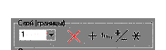
These are editing buttons, affecting the whole layer.

	Erase all data for all profiles in this layer
	Add value from the Value field to all data values in this layer
	Fill all profiles in the layer with value from the Value field, overwriting old data
	Revert data sign for all profiles in the layer
	Multiply data in all profiles in the layer to value from the Value field

Select needed profile from drop-down menu. On the right you can see a group of buttons.

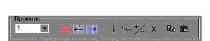
These buttons are for editing data in selected profile.

	Erase all data for all profiles in this layer
	Copy data from current profile to all profiles with smaller ordinal numbers
	Copy data from current profile to all profiles with larger ordinal numbers
	Add value from the Value field to all data values in this profile
	Fill current profile with value from the Value field, overwriting old data
	Revert data sign for current profile
	Multiply data in current profile to value from the Value field
	Copy data from current profile to clipboard
	Paste data from clipboard to current profile

Also, you can manually edit values for each data point. Several shortcuts are provided:

Put a number in any cell in the table and press Tab key. Current profile will be filled with that value.
Put two numbers in any two cells and press Tab key. The range between the two cells will be filled with interpolated data, cells before the first will be filled with first value, and after the second – with the second value.

Switch between text mode and graphic mode editing. In graphic mode, data will be plotted and dragging the point with the mouse can change value for any point. Layer, profile, pint number and value are indicated in the status line.

Calls the Array Operations window. You can add, subtract and copy arrays. If size of the arrays differ, the size of the resulting array will be smallest of the two.

Adding arrays: select from the drop-down list array for storing results and arrays which should be added, then click once.

Subtracting arrays: select from the drop-down list array for storing results and arrays participating in the operation, then click once.

Copying arrays is similar to adding, only you don’t need to select the second array.

Calls the Layer Break window. The selected layer will be broken onto two sublayers. The upper sub-layer will be assigned minimal value from all the blocks making up the layer and the bottom sub-layer will receive maximal. Then, a new boundary position will be calculated so that summated magnetic moment from both blocks equaled that from old block.

Working with well logs

The well log is represented as set of blocks, each characterized with bottom boundary and magnetic susceptibility. The upper boundary of the first block coincides with surface and the upper boundaries of other blocks coincide with bottom boundary of upper block.. Blocks beyond bottom boundary of the model are ignored.

To create a well log, activate Logs tab of the main window. Number and user-defined name of the log will be shown in Log field. Click Add to create new log. Edit the name of the log. This name will be shown on all plots. Select the symbol for the log to show on maps from the Designations drop-down. Input the coordinates of the well.

Blocks are created when you click button Add near the Block drop-down list. For each, the following parameters must be set: coordinate of bottom boundary, absolute depth marker (bottom boundary of the well, relative to daylight surface, coordinates below are negative numbers) and magnetic susceptibility.

Working with images

Activate Images tab of the main window to access graphic-related functions. You can make images of the sections, surfaces, plot various parameters, combine several images into one and export them in bmp format. Use Settings->Basic Settings->Graphic and various windows, accessed from Windows menu.

The type of image can be selected from drop-down list on the left. When the type selected, window Graphics: Basic will show parameters related to this type of image. Types of images are:

Surfaces – draws the selected slice of data in color, with or without isolines. You can select the array that needs to be drawn in Arrays drop-down list in window Graphics: Basic. Every array can have several layers. However, only one layer can be drawn at a time, so you will need to select the layer in the Layer drop-down list in window Graphics: Basic. Another option is to draw or not to draw isolines.
Select section – here you can select the direction of the section for imaging and plotting. You will see the map of the research area with the surface of the data you selected earlier. Clicking the left mouse button on the map adds the point to the broken line. The section will be built along this line. Window Graphics: Tools has several convenient buttons:

X	Erase all points in the section
	Erase last point
	Make section along the first profile
	Make section through the first point of all profiles
	Move the line in the direction of the arrows at he distance equal to the number in the field.

Sections – draw a section along the selected broken line. Different task use different arrays of boundary coordinates and medium properties, so you must select arrays that related to current task. For that, use drop-down lists Depths and Properties in Graphics: Basic window. Another option is to draw or not to draw isolines. You can also select the variant of drawing:

Isolines – draw isolines
Layered – each layer will be divided onto two sub-layers, assuming that susceptibilities are constant within those sub-layers. The upper sub-layer will be assigned minimal value from all the blocks making up the layer and the bottom sub-layer will receive maximal. Then, a new boundary position will be calculated so that summated magnetic moment from both blocks equaled that from old block, that is: 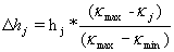; where Dh_j is the thickness of the upper sub-layer, h_j – thickness of j-block before dividing, k_j – susceptibility of j block before dividing and k_max, k_min – maximal and minimal susceptibility in the layer. Thus, “magnetic mass” of two blocks added up will be equal to “magnetic mass” of the block before dividing.
Blocks – this will show blocky structure of model.

Plots – plots various parameters along specified section. Select arrays that you’d like to plot in the drop-down list. All plots will have the same scale and limits will be selected according to the maximal value for all selected arrays. That’s why, for example, plotting simultaneously magnetic susceptibility and boundary coordinates isn’t recommended.
Select section (3D). For building 3D image, you first select two secant planes going through the model and dissecting it onto four rectangular blocks. Click left mouse button to set the intersection axis for these planes. If you’d like not to show one of the four blocks, click right mouse button on one of the rectangles.
Perspective (3D) – builds the 3D image according to selected under “Select section (3D)” parameters. Drag the mouse holding left mouse button to rotate the camera, drag the mouse holding right mouse button to zoom in and out. Settings are similar to that used in section imaging.

Stretch model – scale model along Z-axis proportionally to the parameter
Stretch field – you can draw a magnetic or gravitational field above the model surface. Set this parameter at 0 to draw an image of field on the surface. Set it at negative value to disable drawing the field.
Blocks apart – visually move the blocks away from each other at the specified distance (meters).
Move field up – the height for the drawing of the field from the daylight surface.
Texture quality – use this to adjust the quality of the image. Higher value yields better quality, but requires more resources. It isn’t recommended to exceed 150.
Marks – set the number of tick marks along the coordinate axes.

The Colors window serves for setting up palette. Click the corresponding buttons for setting the colors of isolines, dividers and fonts. Choose the preset palette from the drop-down list. The default is the first one in alphabetic order.

You can switch between “global” and “local” palettes. The local palette assigns colors from minimum to maximum value of plotted parameter. If we change the level of data, the range will automatically change. It is better for making up the details.

The global palette will seek the maximum and minimum values in the entire data cube, so the palette will not be changed from one slice to another.

Click button > to edit the palette. This will call the Edit palette window. You can choose colors, save and load the palettes and work with background textures.

Double-click the element of the palette to change its color and texture.

Point at the element of the palette, press and hold left mouse button, drag the mouse to some other element of the palette and release mouse button. You will be prompted to select the color for the first element, then for the second and after that the range between them will be automatically filled up with a smooth gradation of colors.

When you are satisfied with your palette choices, click Save as… button and save your palette. Click Apply button to see how you picture look with new palette. Clicking Cancel button will cancel the changes and close the Edit palette window. Do not forget to Apply your changes before closing the window, or your changes will be lost.

The Graphics: Basic window will be showing the parameters relevant to drawing the field and horizontal section of the model.

Field – the name of the array you are currently viewing
Relief – the name of the array, which will be visualized as pseudo-relief above the surface of the model
Layer – the number of the layer whose upper boundary will make up horizontal slice; or “Daylight” for the daylight surface.
Shift – the value of the offset for vertical moving of the horizontal slice. Negative – downward.
Marks – set the number of tick marks along the coordinate axes.

You can also select a method for visualizing – blocks, isolines or layers.

Note that after changing image parameters, you should click Refresh button in the main window, or the image could remain the same.

When you are satisfied with image, you’ll probably want to save it for later viewing, embedding in your documents or printing. You can either save the image you currently viewing as Windows Bitmap file, or you can combine several images into one and the save it.

To combine images, use Graphics: Tools window. Click the Remember Image button in this window. Every image will be assigned a number. Select New in the drop-down list to add a new image to the set. After you have acquired a desired number of images, save them by clicking Auto button of the Graphics: Tools window.

To save a single image, use Save to file button of the main window. You will be prompted for filename.

Printing

Printing currently is somewhat delicate matter. For professional printing, we recommend exporting images to specialized packages. You can, however, print a draft for a quick analysis using our package. Click the Print button in the main window. This will call the Print window. You can select printer, adjust orientation justification and zoom and embed a caption in the image. Finally, print the picture clicking the Print button.

Configuration

You can customize many aspects. Use Settings->Basic settings command from the main menu to access customization window.

Interface – customize the user interface

Import check – automatically check the correctness of the data in imported grid file.
Open last file – when started, automatically open last worked file
“Process complete” message – show message window about completion of the computation. Note that while that window is shown, the next job will not be run.
Autosave after compute – automatically save the job after successful computation.

Precision – number of signs after decimal point.

Meters – precision for length-related data
Other – all other, including densities
Lateral units – units for labeling X and Y axes in all the images
Height units – the same for Y axis

Graphics – parameters for visualizing

Interpolation – select methods for the interpolation of data for visualizing surfaces, sections and plots.
Smoothing – use smooth color transits
Line width – width, in pixels, of the lines for drawing plots
Max picture size – the size of preallocated picture buffer. Restart the program after changing these.
Depth shadowing – this should be self-explaining…

File types – register Windows file extensions association
Data path – select the directory, where shared data for the program are located.
Array names – this affects the names of array in all drop-down lists in the program. You can change the name of the array, types of tasks and position of the array in the list. Click the line with the array name to see the description of the array.

Do not forget to Apply your changes before closing the window.

Importing data from grid file

The format of the grid file is simple. It is a plain ASCII text file containing columns of numbers. First and second columns are considered X and Y coordinates of data points, all other are values of data. Use command File->Import and browse for the file. Data will be checked for consistency (if this option isn’t turned off in the settings). If all goes well, you will see window with 3D preview of data at the lower right. The preview can be rotated with the mouse. Select the columns of data and arrays for storing the data. The number of profiles and points will be computed automatically (that’s why it is important to have X and Y coordinates in the file). Click Create arrays. This will create arrays of needed size, but will not store the data. You must click Apply to store imported data in the arrays.

Note that data points must be uniformly distributed along the rectangular grid. Non-numeric symbols are not allowed in the file. A newline must be the last symbol in the file.

Troubleshooting

ü Program does not start. Possible reasons:

o Read-only attribute set on the files. Remove it.

o Too large max size of the picture specified in settings. Remove *.ini file in the program directory to reset all settings to defaults.

o Some files are missing or corrupted. Reinstall the program.

o Close all non-needed applications. Reboot Windows.

ü Other errors do not exist, and if you’ll find them, do not believe your eyes.

^[1] The number of layers and blocks in the layer is, in fact, limited by physical memory available. For example, during the creation of the model of 1000x1000x1000 73 Gb of memory required only for storing the model. Additionally no more than 8 mb. of memory is required for the solution.